Feature Importance on MNIST with feature counts
Select a subset of 3’s and 5’s from MNIST
Here we train a forest using RerF with the RandMatImagePatch
option with patch.min = 1 and patch.max = 5.
## Get a random subsample, 100 each of 3's and 5's
threes <- which(mnist$Ytrain %in% 3)
fives  <- which(mnist$Ytrain %in% 5)
numsub <- c(threes, fives)

Ytrain <- mnist$Ytrain[numsub]
Xtrain <- mnist$Xtrain[numsub,]
Ytest <- mnist$Ytest[mnist$Ytest %in% c(3,5)]
Xtest <- mnist$Xtest[mnist$Ytest %in% c(3,5),]
# p is number of dimensions, d is the number of random features to evaluate, iw is image width, ih is image height, patch.min is min width of square patch to sample pixels from, and patch.max is the max width of square patch
p <- ncol(Xtrain)
d <- ceiling(sqrt(p))
iw <- sqrt(p)
ih <- iw
patch.min <- 1L
patch.max <- 5L

forestS <- RerF(Xtrain, Ytrain, num.cores = numCores, FUN = RandMatImagePatch,
               paramList = list(p = p, d = d, iw = iw, ih = ih,
                                pwMin = patch.min, pwMax = patch.max), max.depth = 8)

predS <- Predict(Xtest, forestS, num.cores = numCores)
(mnist.error.rate <- mean(predS != Ytest))
## [1] 0.01892744
forestRerF <- RerF(Xtrain, Ytrain, num.cores = numCores, FUN = RandMatBinary,
               paramList = list(p = p, d = d), max.depth = 8)


predRerF <- Predict(Xtest, forestRerF, num.cores = numCores)
(mnist.error.rate <- mean(predRerF != Ytest))
## [1] 0.02208202
forestRF <- RerF(Xtrain, Ytrain, num.cores = numCores, FUN = RandMatRF,
               paramList = list(p = p, d = d), max.depth = 8)


predRF <- Predict(Xtest, forestRF, num.cores = numCores)
(mnist.error.rate <- mean(predRF != Ytest))
## [1] 0.02050473
system.time({
FeatImpS <- FeatureImportance(forestS, num.cores = numCores, type = "C")
})
## Message: Computing feature importance as counts of unique feature combinations.

##     user   system  elapsed
## 1229.062    6.560  314.241
ni <- matrix(0, length(FeatImpS$features), ncol(Xtrain))

for(i in 1:length(FeatImpS$features)){
  ni[i, FeatImpS$features[[i]]] <- FeatImpS$imp[i]
}

NN <- matrix(apply(ni, 2, sum) / nrow(ni), 28, 28, byrow = FALSE)
saveRDS(NN, file = "NNsrerf.rds")

system.time({
FeatImpRerF <- FeatureImportance(forestRerF, num.cores = numCores, type = "C")
})
## Message: Computing feature importance as counts of unique feature combinations.

##     user   system  elapsed
## 1750.585   11.082  444.860
nir <- matrix(0, length(FeatImpRerF$features), ncol(Xtrain))

for(i in 1:length(FeatImpRerF$features)){
  nir[i, FeatImpRerF$features[[i]]] <- FeatImpRerF$imp[i]
}

NNr <- matrix(apply(nir, 2, sum) / nrow(nir), 28, 28, byrow = FALSE)
saveRDS(NNr, file = "NNrerf.rds")

system.time({
FeatImpRF <- FeatureImportance(forestRF, num.cores = numCores, type = "C")
})
## Message: Computing feature importance as counts of unique feature combinations.

##    user  system elapsed
##  14.579   0.323   5.549
nirf <- matrix(0, length(FeatImpRF$features), ncol(Xtrain))

for(i in 1:length(FeatImpRF$features)){
  nirf[i, FeatImpRF$features[[i]]] <- FeatImpRF$imp[i]
}

NNrf <- matrix(apply(nirf, 2, sum) / nrow(nirf), 28, 28, byrow = FALSE)
saveRDS(NNrf, file = "NNrf.rds")
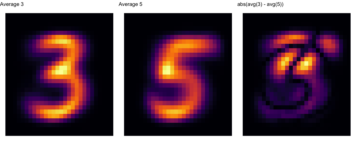
plot the average 3 and 5 from the training set
the3s <- Xtrain[Ytrain == 3, ]
the5s <- Xtrain[Ytrain == 5, ]

sum3 <- matrix(apply(the3s, 2, sum) / sum(Ytrain == 3), 28, 28, byrow = FALSE)
sum5 <- matrix(apply(the5s, 2, sum) / sum(Ytrain == 5), 28, 28, byrow = FALSE)

g <- expand.grid(x = 1:28, y = 1:28)
gg <- rbind(g, g)

nn <- as.vector(t(NN[28:1, ]))
nnrerf <- as.vector(t(NNr[28:1, ]))
nnrf <- as.vector(t(NNrf[28:1, ]))

s3 <- as.vector(t(sum3[28:1,]))
s5 <- as.vector(t(sum5[28:1,]))
s3m5 <- abs(s3 - s5)

Z <- data.frame(g, weight = c(nn, nnrerf, nnrf, s3, s5, s3m5), Alg =  rep(c("MF", "Sporf", "RF", "Average 3", "Average 5", "x3m5"), each = length(nn)))

sc0 <- scale_fill_gradientn(colours = viridis(255))
sc1 <- scale_fill_gradientn(colours = inferno(255))

a1 <- ggplot(data = Z[ Z$Alg == "Average 3",    ], aes(x = x, y = y, fill = weight)) + geom_raster() + theme_void() + guides(fill = FALSE) + sc1 + ggtitle("Average 3")
a2 <- ggplot(data = Z[ Z$Alg == "Average 5", ], aes(x = x, y = y, fill = weight)) + geom_raster() + theme_void() + guides(fill = FALSE) + sc1 + ggtitle("Average 5")
a3 <- ggplot(data = Z[ Z$Alg == "x3m5", ], aes(x = x, y = y, fill = weight)) + geom_raster() + theme_void() + guides(fill = FALSE) + sc1 + ggtitle("abs(avg(3) - avg(5))")

grid.arrange(a1, a2, a3, ncol=3)
#ggslackr(grid.arrange(a1, a2, a3, ncol=3), channels="#manifold-forest")
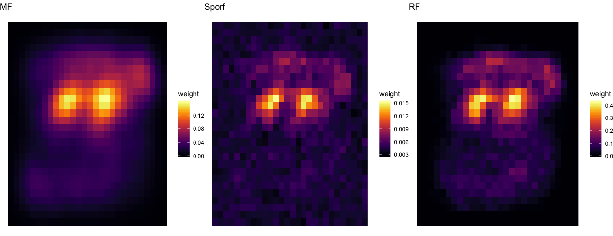
Feature heatmap
These are the features that S-RerF and RerF used, plotted as averaged heatmaps.
p1 <- ggplot(data = Z[ Z$Alg == "MF",    ], aes(x = x, y = y, fill = weight)) + geom_raster() + theme_void() + sc1 + ggtitle("MF")
p2 <- ggplot(data = Z[ Z$Alg == "Sporf", ], aes(x = x, y = y, fill = weight)) + geom_raster() + theme_void() + sc1 + ggtitle("Sporf")
p3 <- ggplot(data = Z[ Z$Alg == "RF",    ], aes(x = x, y = y, fill = weight)) + geom_raster() + theme_void() + sc1 + ggtitle("RF")

grid.arrange(p1, p2, p3, ncol=3)